confocaloid wrote: March 22nd, 2025, 7:50 am
What would be a good, reliable algorithm for automatically computing the number of 'apparent turns' of a "beyblade" object (an oscillator or spaceship)?
This is a only a partial answer to this question but includes a proof of concept for a proposed method of detecting the number of apparent turns.
The first part of the analysis to determine period and displacement of any beyblade like pattern is I think already pretty well covered by existing tools and I won't cover it here, but will assume the results can be determined for any given pattern.
The general idea to determine number of apparent turns is this:
- Choose a starting generation to use as reference - can be arbitrary for "well behaved" beyblades. Not sure how to approach beyblades with erratic behaviour because it would be necessary to select a generation which appears to repeat. Maybe: repeat this whole process for multiple reference generations, OR detect a "compact", low population generation and use that.
- Calculate the peak 2D cross correlation of the reference generation with all generations in one period. The cross correlation window should cover an area large enough to move the window as far as the furthest apparent motion. This can be achieved by doing a full cross correlation, or by tracking movement of the "centre of gravity" of the pattern across one whole period.
- From the timeseries of peak cross correlation, determine the number of apparent turns by counting peaks. This can by done with an FFT analysis (at least for "well behaved" beyblades (as shown in proof of concept below). For less regular beyblades a robust peak finding algorithm may give a decent result, but it's always hard to know if all the peaks that are "intereting" will be detected, and all the noise rejected. I didn't explore this technique here but there's a lot of good literature (and code) on the topic.
I wrote some code to test this idea with the beyblade posted above. It's in MATLAB because that's what I had to hand but shouldn't be to hard to understand and/or convert to Python (preferably with numpy). Note that MATLAB uses 1-based indexing and matrix indices are by row, then column.
Code: Select all
%% Sample rle pattern conversion

% bb_header0 = 'x = 35, y = 35, rule = R12,C10,S59-117,200-488,B89-114,155-170,400-488,NC';
bb_rle0 = ['16.6A$14.11A$13.14A$12.8A2B6A$12.5A7B5A$11.5A10B4A$11.4A12B3A$10.4A5B', ...
'8C4A$10.4A4B10C4A$9.5A4B4C5D2C4A$9.6A3B3C8DC3A$9.6A3B3C9D4A$9.7A3B2C3D', ...
'3E4D3A$10.7A2B2C2D6E2D2AB$11.7ABC2D8E2D2B$12.7AB2D3E3F3ED2B$2.I11.6AD', ...
'2E6F3E2B$.2I11.6ADE8F2E3B$3I11.6AE9F2E3B$3I12.5AF6G3FE2BC$3I12.2IA10G', ...
'3FB2C$3I13.2I3H7G3F3C$3I14.2I5H4G3F3C$.I2H13.4I4H3G3F3C$.3H13.4I4H3G2F', ...
'3C$.4H13.4I3H3GF4C$2.4H12.4I3H3GF3D$2.4HG11.4I3H3G3D$3.3H2G9.5I2H3G4D', ...
'$4.2H3G7.5I3H2G4D$6.4G10I3HGE4D$7.5G6I3H6ED$8.4G6F9E$10.2G7F5E$12.8FE!'];

rule = 'R12,C10,S59-117,200-488,B89-114,155-170,400-488,NC';
range = 12;
n_states = 10;
sz_x = 35;
sz_y = 35;
beyblade_cells0 = rle_decode(bb_rle0, [sz_x, sz_y]);
period = 884;

pad = range+5; % 5 is arbitrary, allows for movement outside of initial BB
ngrid = 35+pad*2;
cells0 = zeros(ngrid,ngrid);
cells0(pad+(1:sz_x), pad+(1:sz_y)) = beyblade_cells0;

%% Evolve pattern and test cross correlation
% Use original pattern as reference
% Normalise to scale of 1->2 with live cells -> 2 and dead cells -> 1
rescale = @(v)2-mod(v-1, n_states)/(n_states-1);
cells_ref = rescale(beyblade_cells0);

cells2 = cells0;
% Initialise array for results
%   row 1 -> x offset of peak cross correlation
%   row 2 -> y offset of peak cross correlation
%   row 3 -> peak cross correlation
xcorr_res = zeros(3, period);

for ii = 1:period
    cells2 = evolve_ltl(cells2, rule);
    xcorr_pad = 5; % Adjust this according to apparent movement of the core
    xcorr_idxs = 1+pad-xcorr_pad:sz_x+pad+xcorr_pad; % Assumes sx_y == sx_x
    xcorr = conv2(rescale(cells2(xcorr_idxs, xcorr_idxs)), rot90(rot90(cells_ref)), 'valid');
    [m, mi] = max(xcorr, [], 'all');
    [ri, ci] = ind2sub(size(xcorr), mi);
    xcorr_res(:, ii) = [ri-xcorr_pad-1; ci-xcorr_pad-1; m];
end

%% Plot cross correlation results and FFT of peak xcorr values
figure()
tiledlayout(3,1)
nexttile
plot(1:period, xcorr_res(1:2,:))
title('x and y offsets of cross correlation peak')
nexttile
plot(1:period, xcorr_res(3,:))
title('cross correlation peak by generation for one period')
nexttile
Fs = 1; % Sample rate, arbitrarily set to 1 gen/s
% T = 1/Fs;
L = period;
F = fft(xcorr_res(3,:)); % DFT using fast fourier transform
F(1) = 0; % Set DC component to 0
freq = Fs/L*(0:L-1);
plot(freq, abs(F)) % plot the magnitude of the complex fft spectrum
[peak, f_idx] = max(abs(F));
xlabel('frequency')
title('Amplitude of fft spectrum of the peak cross correlation')
disp([f_idx-1, freq(f_idx), 1./freq(f_idx), period*freq(f_idx)])
rle_decode is a function to convert rle to a matrix of cell states
evolve_ltl is a function to evolve a pattern in this particular LTL rule
The result displayed at the end is: "57.0000 0.0645 15.5088 57.0000".
f_idx works out to be what we want because the sampling rate is treated as 1 per second so it's the length of frequency vector (884) multiplied by the dominant frequency, but the most reliable result is probably obtained from the last value "period*freq(f_idx)"
The output from the plots looks like this:
Note the x and y offsets jump around a bit - there's a dependence on the xcorr_pad value and the scaling parameters used. the jump corresponds to relative shifts in the location of the peak cross correlation when the beyblade is near 180deg rotated from the reference pattern.
Also, ignore the half of the frequency graph > 0.5. That corresponds to the negative frequency side of the dual sided DFT which I didn't bother to wrap around or truncate.

- beyblade_analysis.png (111.73 KiB) Viewed 5176 times
Edit: Updated FFT analysis code to be a little more rigorous and corresponding update to beyblade analysis image
Edit 2: Correct mixup in FFT frequency interpretation code (off-by-one strikes again)